A Machine Learning Program/Model that makes decisions just like the human brain.

How does it do it?

When we think, we subconciously give priority to some thoughts and decisions in our brains, we identify events, and arrive at a conclusion.

Neural Networks act in the same pattern, giving weight, identifying phenomenons, and arriving at a conclusion or conclusions.

Neural Networks can be classified as being made up of three layers:

Input Layer: Receives the input data, which could be images, sound waves, or text.

Hidden Layers: One or more layers that perform complex representations of the input data, allowing the network to learn and adapt.

Output Layer: Generates the final prediction or output, based on the inputs and transformations applied by the hidden layers. In the layers, nodes, or in brain terms, neurons, exist, and have their own weights, thresholds. If outputs of individual nodes are beyond the threshold, they send data to the next layer of the network, otherwise no action is undertaken.

Neural Networks quite literally learn, just like how a human learns, from training.

Training data is provided, and the Network learns and becomes more accurate over time and tries.

The Math Behind Neural Networks:

Each node or neuron in the network applies a weighted sum of its inputs, followed by an activation function, to produce an output. The formula for this process is:

output = activation_function(weighted_sum(inputs))

The weighted sum is calculated as:

weighted_sum = Σ(input_i * weight_i) + bias

where input_i is the input from the previous layer, weight_i is the learned weight for that input, and bias is a constant term.

Activation Functions: Sigmoid and ReLU:

Activation functions give non-linearity to the network, making it learn complex relationships between inputs and outputs. Two commonly used activation functions are:

Sigmoid:

Maps the input to a value between 0 and 1, using the formula:

sigmoid(x) = 1 / (1 + exp(-x))

ReLU (Rectified Linear Unit):

Maps all negative values to 0 and all positive values to the same value, using the formula:

relu(x) = max(0, x)

Just like humans, Neural Networks learn through a process of trial and error, refining their skills with each experience. This iterative process is called backpropagation, where the network adjusts its weights and biases to minimize the gap between predictions and reality.

The Learning Loop

Imagine a child learning to ride a bicycle. At first, they may fall down, may not understand how to turn or how to brake. But with more and more practice, they get to know the timing, understand when and how to brake, and how to turn etc. Similarly, Neural Networks follow this learning loop:

Prediction: The network makes a prediction based on its current weights and biases.
Error Calculation: The difference between the prediction and the actual output is calculated, highlighting the network’s mistakes.
Adjustment: The network adjusts its weights and biases to reduce the error, just like the child gets to understand the timings of braking and turning .
Repeat: Steps 1–3 are repeated, with the network refining its predictions and reducing errors with each loop.

The Practice Schedule:

Just as a practice schedule helps you improve the child’s bike riding, optimization algorithms guide the network’s learning process. Popular algorithms like Stochastic Gradient Descent (SGD), Adam, and RMSProp adjust the learning rate, momentum, and other parameters to better the network’s performance.

Convergence:

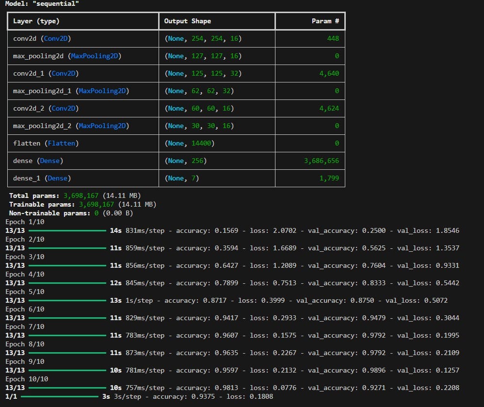
A CNN Model of mine with 93.75 accuracy at the end (Adam algorithm)

As the network iterates through the learning loop, it converges towards the optimal set of weights and biases, making minimal errors and maximizing accuracy. This is like mastering riding the bike, where turning, braking and pedalling all are easy and perfect.

Conclusion:

Neural Networks are powerful tools for Machine Learning, enabling machines to learn from data and make predictions or decisions. By understanding the mechanics and math behind these networks, we can unlock their full potential and apply them to a wide range of applications, from image recognition to natural language processing and further on with Deep Learning and the like.

Citations:

IBM:

https://www.ibm.com/topics/neural-networks

University Of Michigan: http://web.eecs.umich.edu/~jabernet/eecs598course/fall2015/web/notes/lec15_110315.pdf